rm(list=ls())
df <- read.csv('https://www.dropbox.com/scl/fi/8sf5s4uloq8rgu0tbf45y/sco_prem_2024.csv?rlkey=qvoewxn2nd1f6clqbwo0aib7f&dl=1')90 Week Ten Practical
Agenda
Review Introduction.
Review Clustering.
Review Dimensionality reduction.
Practice cluster analysis
Review Ensemble methods.
Demonstration of Neural Networks.
Practical demonstration - SCO 2023-24.
90.1 Cluster analysis - practice
Download the dataset available here:
Take some time to figure out what the variables might reflect.
Use the following code to select the variables you wish to explore via cluster analysis, and scale those variables.
# For example....

selected_data <- scale(df[, c("home_team_win_ratio", "away_team_win_ratio", "home_team_points_ratio", "away_team_points_ratio")])
Now, conduct a k-means cluster analysis using k=3.
First, conduct the cluster analysis.
Then, create a PCA analysis for dimensionality reduction.
Create a dataframe with the principal components and cluster assignment.
Plot the first two PC components.
Assign cluster allocation to the observations in the original dataset.
Review the gap score to check the optimum number of clusters.
Repeat the cluster analysis with an alternative number of clusters (k), based on the gap score.
Finally, review the cluster allocations. What do they tell you about the observations?
show solution
k <- 3

set.seed(123)

#-----------------------
# Perform cluster analysis
#-----------------------

clusters <- kmeans(selected_data, centers = k, nstart = 25)
#-----------------------
# Perform PCA
#-----------------------
pca_result <- prcomp(selected_data)

#-----------------------
# Create data frame with PCs and cluster assignments
pca_data <- data.frame(pca_result$x[, 1:2], Cluster = clusters$cluster)

#-----------------------
# Plotting the first two principal components
#-----------------------
plot(pca_data[,1], pca_data[,2], col = pca_data$Cluster, pch = 20, xlab = "Principal Component 1", ylab = "Principal Component 2", main = "K-Means Clustering with PCA")

points(clusters$centers[, 1:2], col = 1:k, pch = 8, cex = 2)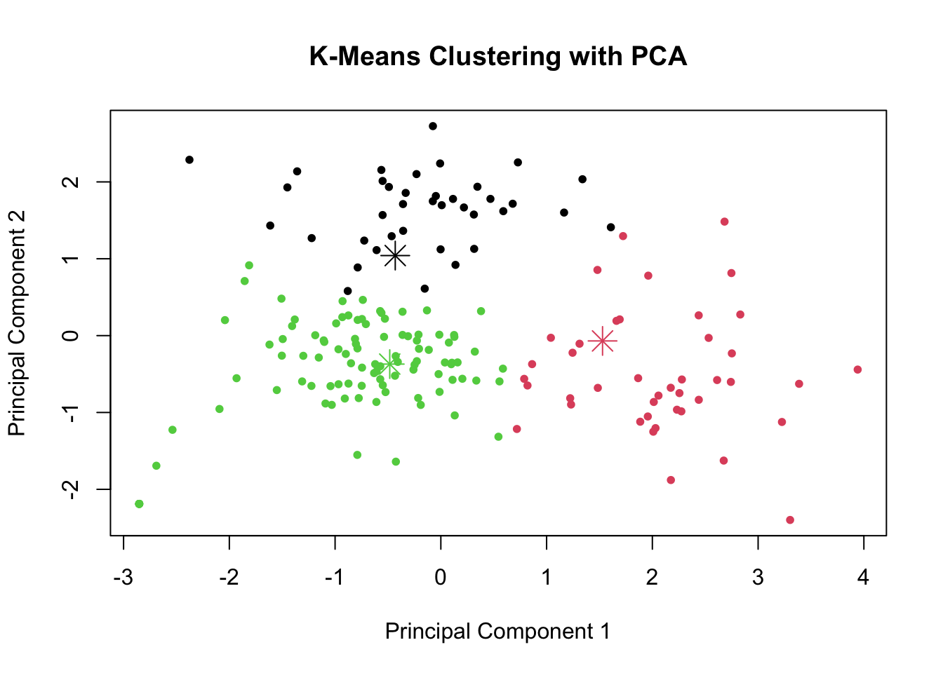
show solution
#-----------------------
# Check n clusters
#-----------------------
library(cluster)
gap_stat <- clusGap(selected_data, FUN = kmeans, nstart = 25, K.max = 10, B = 50)
plot(gap_stat, main = "Plot of Gap Statistic")

#-----------------------
# Adding the cluster assignments to the original dataframe
#-----------------------
df$Cluster <- clusters$cluster

#-----------------------
# Examine features of the clusters
#-----------------------
library(ggplot2)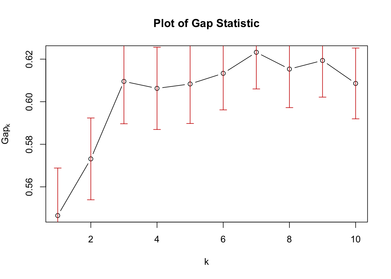
show solution
# Using ggplot2 to plot home_team_win_ratio by cluster
ggplot(data = df, aes(x = Cluster, y = home_team_win_ratio, group = Cluster)) +
  geom_point() +  # Add points
  geom_line() +   # Connect points within each cluster with lines
  theme_minimal() +  # Use a minimal theme
  labs(x = "Cluster", y = "Home Team Win Ratio", title = "Home Team Win Ratio by Cluster")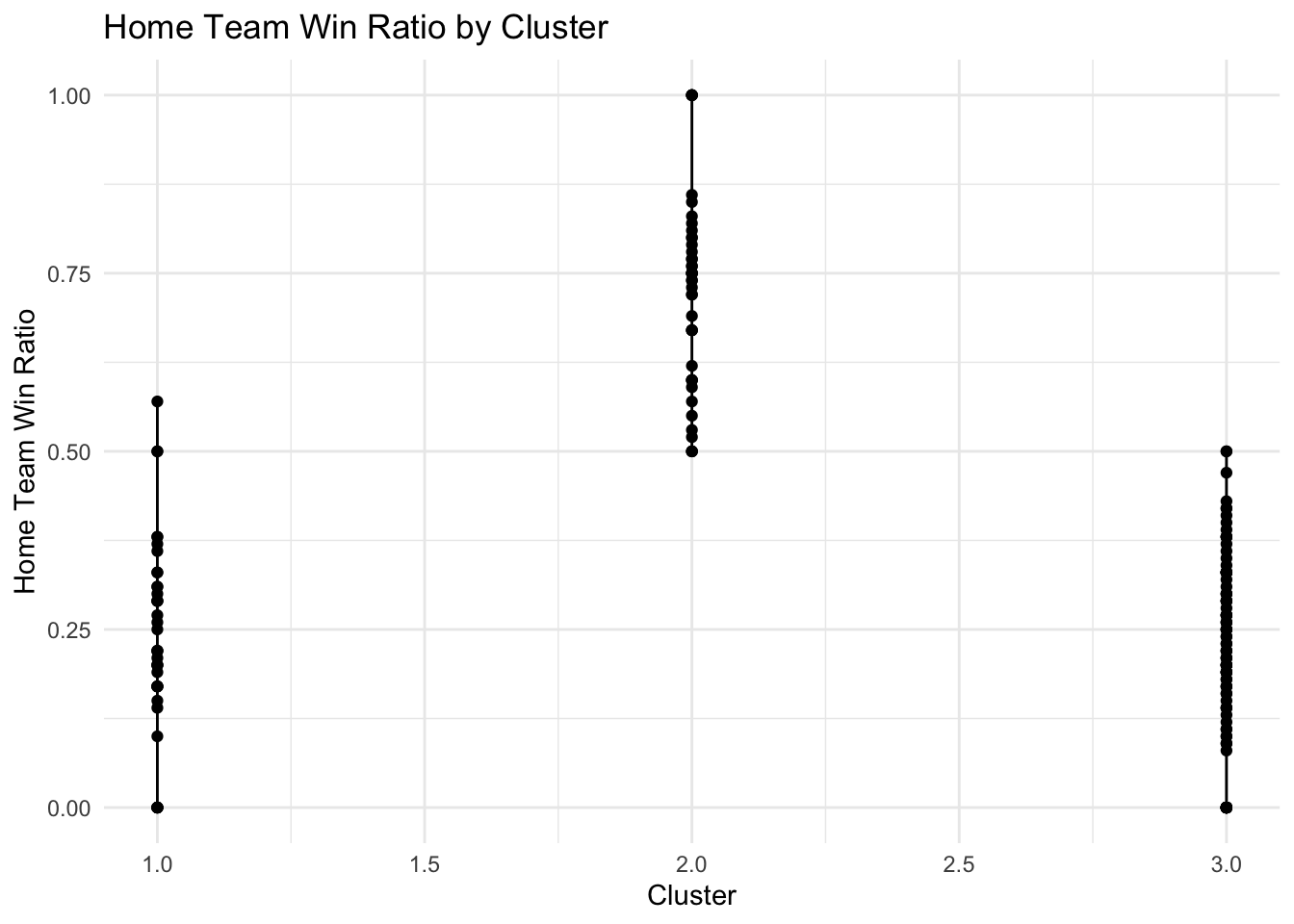
show solution
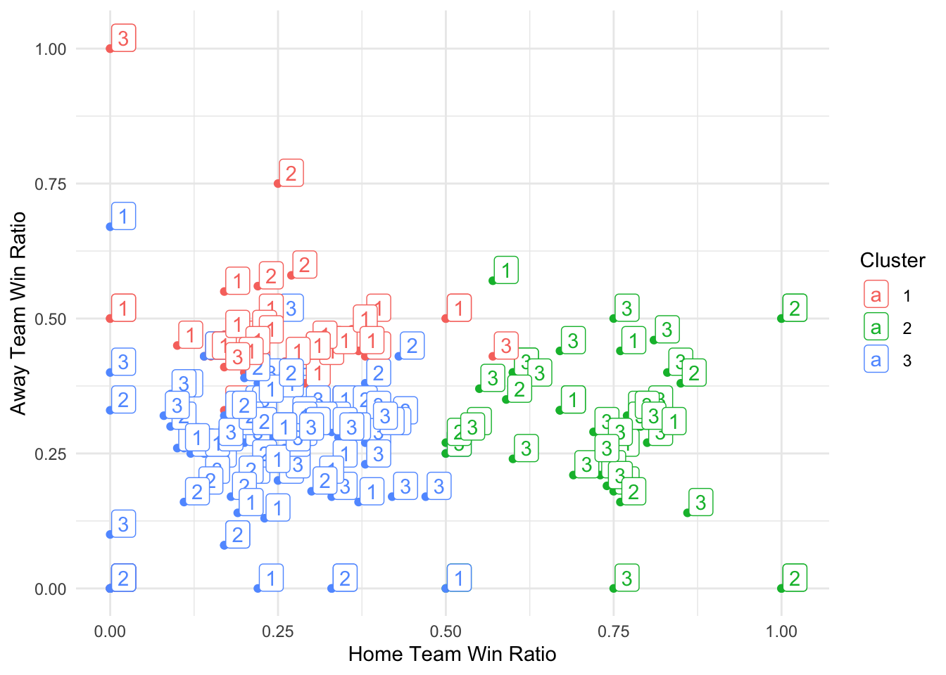
# Create scatter plot
ggplot(data = df, aes(x = home_team_win_ratio, y = away_team_win_ratio, color = factor(Cluster))) +
  geom_point() +
  labs(x = "Home Team Win Ratio", y = "Away Team Win Ratio", color = "Cluster") +
  theme_minimal()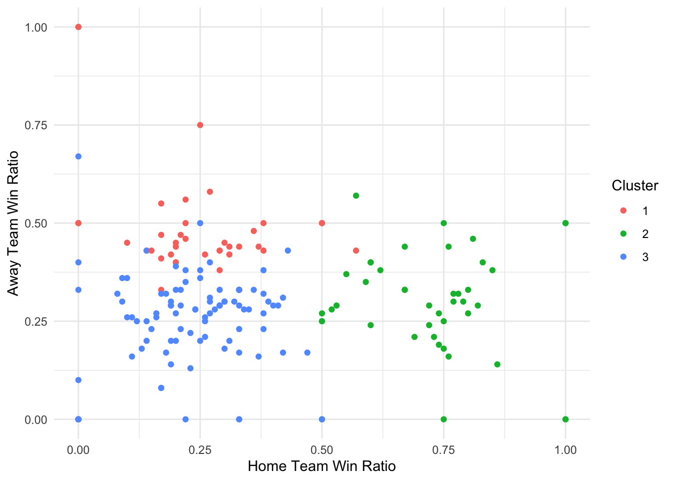
show solution
# Load the ggplot2 package
library(ggplot2)

# Create the scatter plot with labels
ggplot(data = df, aes(x = home_team_win_ratio, y = away_team_win_ratio, color = factor(Cluster))) +
  geom_point() +
  geom_label(aes(label = result_category), nudge_y = 0.02, nudge_x = 0.02) +  # Nudge positions labels slightly to avoid overlap
  labs(x = "Home Team Win Ratio", y = "Away Team Win Ratio", color = "Cluster") +
  theme_minimal()